An introduction to Markov Chain Monte Carlo (MCMC)
MCMC Basics
Suppose we want to sample from a (Boltzmann) probability distribution of the form $\pi(x) = \frac{1}{Z} e^{-\beta U(x)}$, where $ U(x) $ is a potential energy function and $ Z $ is the normalizing constant. $\beta$ is an inverse temperature, but it will be kept constant for the purposes of this article, so don’t worry about it. This is a common problem in statistical physics, machine learning, and many other fields. However, sampling from this distribution can be challenging, especially when $U(x)$ is complex and high-dimensional.
Let’s start with a simple example. Suppose we have two states in one dimension separated by an energy barrier. Below, we’ll picture both the energy and the probability density induced by the Boltzmann distribution.
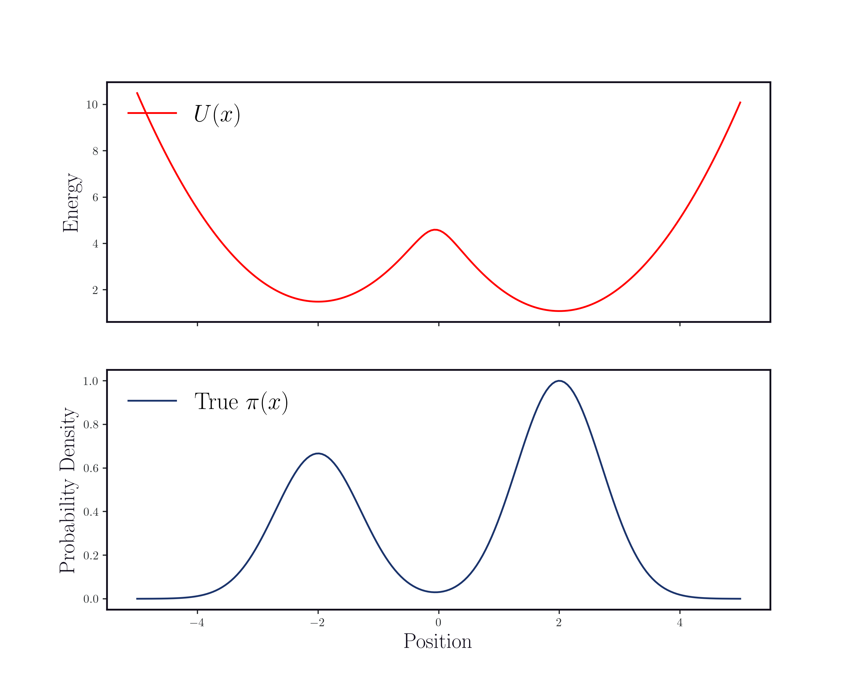
In most use cases, we don’t have access to the normalizing constant $Z$, but we do have access to $U$. You can think about this as being able to evaluate an energy, but only evaluating relative probabilities: say we’re comparing state $x$ and state $x’$, then
$\frac{\pi(x’)}{\pi(x)} = \frac{ Z^{-1} \exp (- \beta U(x’))}{Z^{-1} \exp (- \beta U(x))} = \exp (- \beta U(x’) + \beta U(x))$
The ability to compare the relative probabilities of two states allows us to use a class of sampling algorithms called Markov Chain Monte Carlo (MCMC). The basic idea is to set up a set of random ‘moves’ that will always go down in energy when possible, but occasionally go up in energy. This leads to having more samples in lower energy states, but still a few in higher energy states. If you collect enough samples from this process, you end up with a set of $x$ values whose coordinates are distributed according to $\pi(x)$; which we write using the notation $x \sim \pi(\cdot)$.
To actually implement this algorithm, you need a proposal distribution which we call $q$. This just gives you a way to propose the next state $x’$, given that you are currently at state $x$, and we have to also know its probability density $q(x’ \mid x)$.
The exact algorithm balances this property of going to lower energy states more often with the bias induced by your proposal distribution: if you’re really likely to go from state $x$ to $x’$ under $q$, you’ll want to occasionally reject a lower energy transition to correct for the bias in your proposal. The exact algorithm implements is as follows:
\begin{algorithm}
\caption{Basic MCMC}
\begin{algorithmic}
\Require Initial coordinates $x_0$, energy function $U(x)$, inverse temperature $\beta$, easy-to-sample proposal distribution $q(x' \mid x)$, number of simulation steps $T$, burn-in time $b$ \\
\FOR{$t \in \{1, \dots, T\}$}
\STATE Sample proposal $x' \sim q(\cdot \mid x_t)$
\STATE Compute $\alpha = \frac{\pi(x')}{\pi(x_t)} \frac{q(x_t \mid x')}{q(x' \mid x_t)} = \exp(-\beta U(x') + \beta U(x_t)) \frac{q(x_t \mid x')}{q(x' \mid x_t)}$
\STATE Sample uniform random $u \in [0,1]$
\IF{$u < \alpha$}
    \STATE $ x_{t+1} \gets x' $
\ELSE
    \STATE $ x_{t+1} \gets x_t $
\ENDIF
\ENDFOR
\RETURN $ \{ x_t \}_{t=b}^T $
\end{algorithmic}
\end{algorithm}
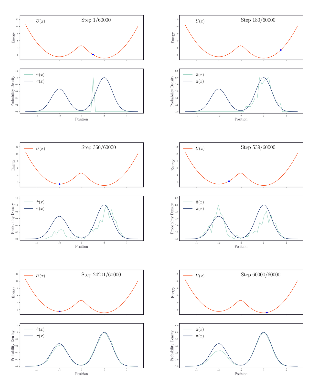
We can implement this on our example distribution with modes at $x=-2$ and $x=2$ and using a gaussian proposal distribution $q(x’ \mid x) = \mathcal{ \cdot ; x, \sigma}$ where $\sigma$ sets the scale of the perturbation. Here is an example trajectory, showing the empirical probability distribution we collect on the bottom.
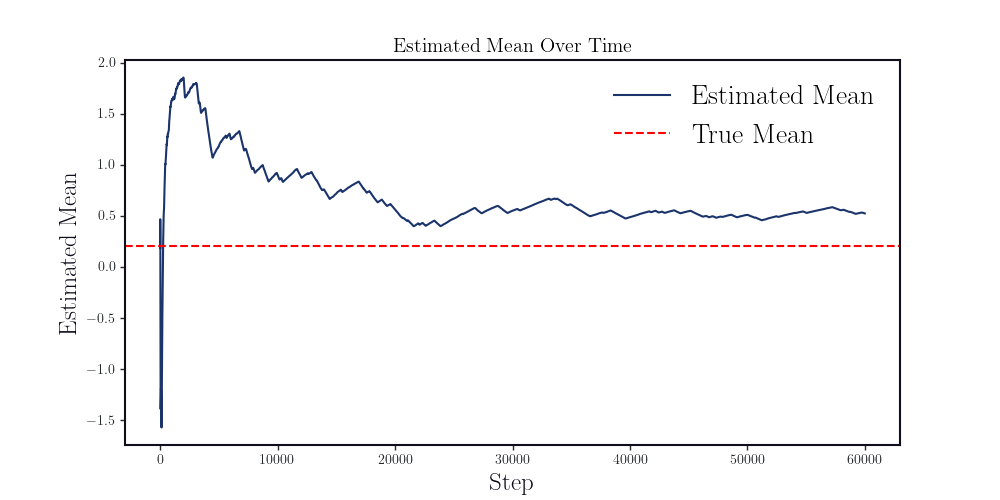
Using these samples, let’s calculate the true mean value of $x$ under the distribution $\pi$. This can be a high-dimensional integral in general, so it’s useful to use the Monte Carlo samples as an estimator: $\mu = \int x \cdot \pi(x) dx \approx \frac{1}{N} \sum_{i=1}^N x_i ; > x_i \sim \pi(\cdot)$ where our samples come from the MCMC chain. The longer we run the chain, the closer we get to the ground truth value:
Now suppose we separate these modes even further, placing them at $x=-4$ and $x=4$. Let’s see what happens when we try to run the same code:
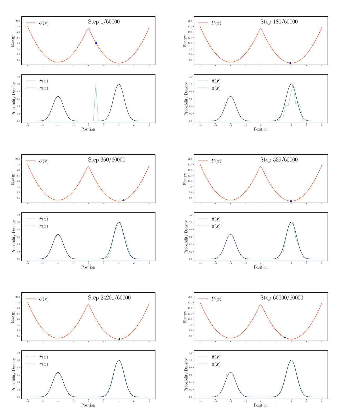
Annoyingly, we start off in the righthand mode and never seem to escape it! This gives us a good local estimate of the mode density, but we don’t see anything about the second mode. Let’s try again to see the mean estimate over time:
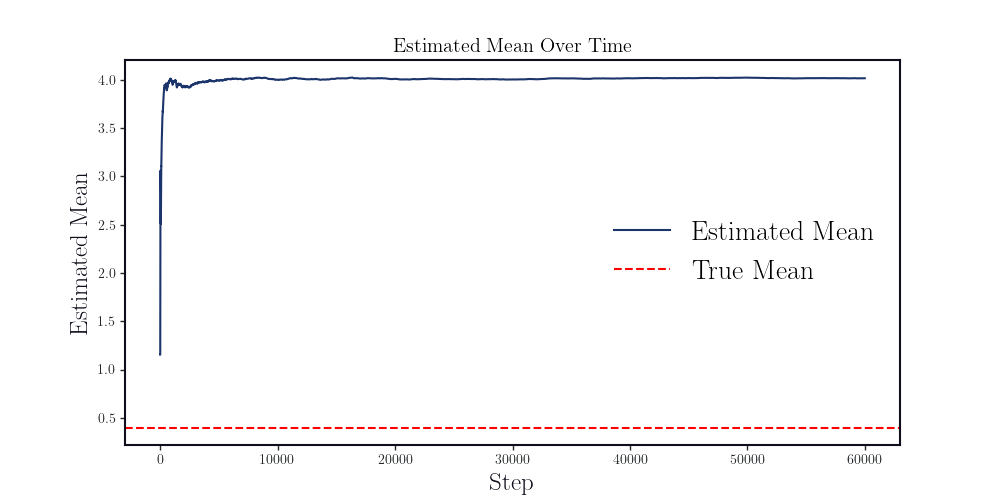
As you can see, our estimate is very bad. The lesson is that local MCMC moves have trouble climbing energy barriers. In the first example the energy barrier was low enough that this didn’t cause a problem, but when we move the modes further apart (which in turn heightens the energy barrier), you end up with mode collapse which is highly sensitive to your starting conditions.
One remedy to this issue is to use a global proposal distribution, which does not depend on the previous state. In this example we’ll look at $q(x’ \mid x) = q(x’) = \mathcal{N}(0, 4)$, which is a gaussian distribution centered at the origin with variance $4$. Note that each proposed state $x’$ does not actually depend on the previous state $x$
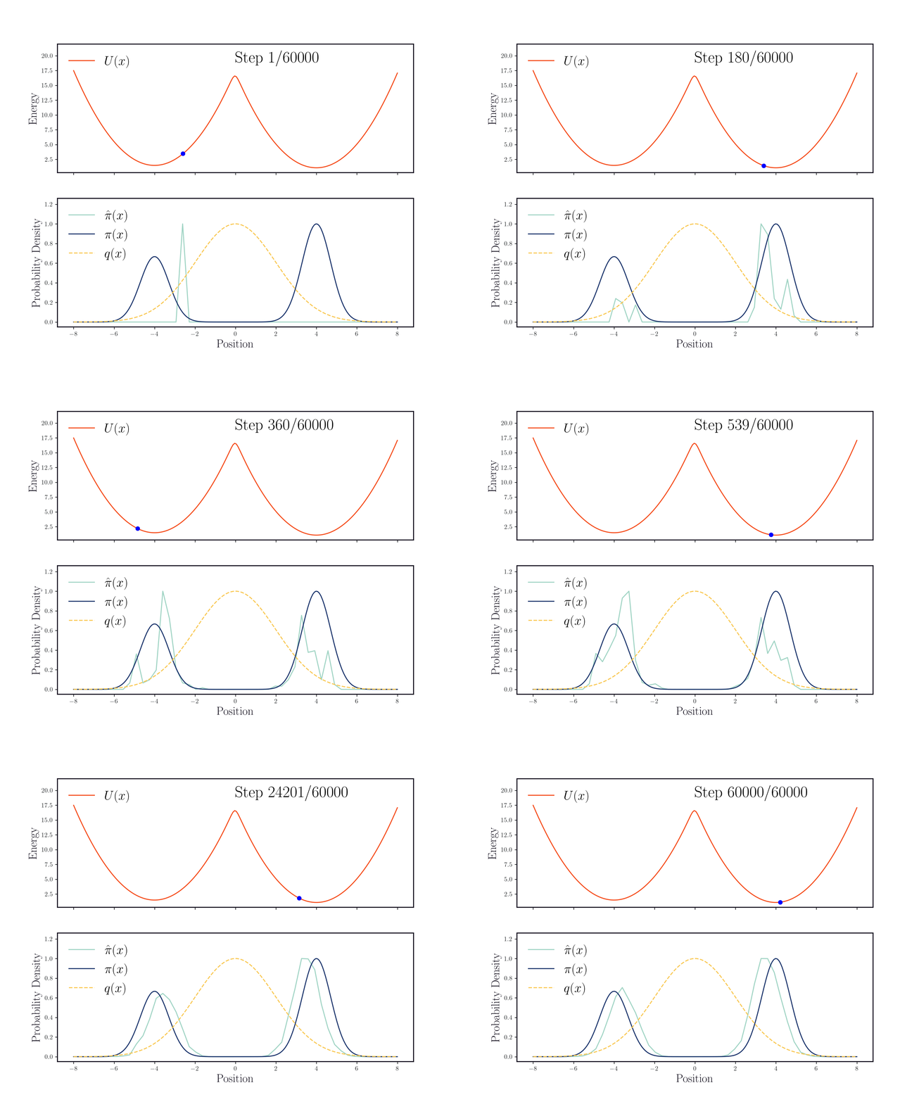
Notice how the points are allowed to ‘teleport’ to the other side. However, we still reject a lot of the proposed configurations because we are essentially wasting proposals on the area in the middle where there is high proposal probability and low target probability.–lgov7h